GPT3-学习笔记

GPT3

摘要

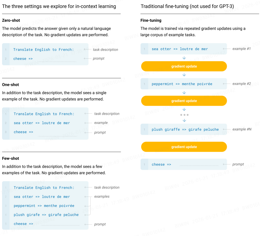
大模型区别于传统机器学习的一项**关键能力**，是能够通过极少的示例（Few-shot Learning）快速理解并执行新任务。**这一能力在GPT-3上取得了里程碑式的突破**。其发表于2020年的论文《Language Models are Few-Shot Learners》首次系统性地证明：当模型规模达到千亿参数（175B）时，无需针对特定任务进行微调，仅通过在提示中提供几个示例，就能达到接近传统监督学习的性能，这被称为**上下文学习（In-Context Learning）**。

• GPT3论文链接 https://arxiv.org/abs/2005.14165


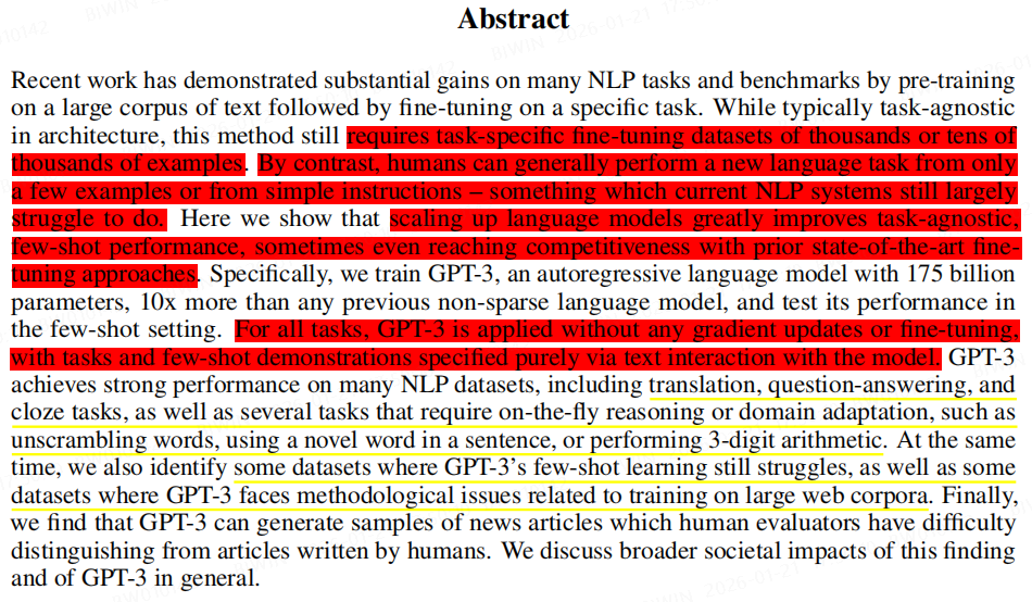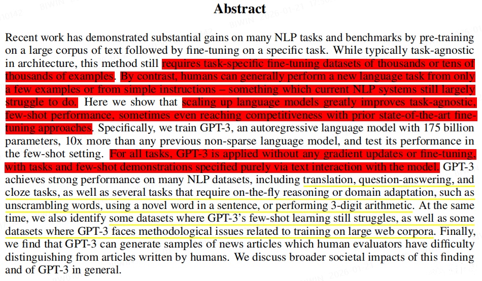
下面内容具体解释下Abstract中提到的：

1. scaling up language models

2. gradient updates

3. few-shot (only a few examples or from simple instructions)

参数量

从GPT-1到GPT-3，其核心思路始终如一：基于Transformer架构，在海量无标注文本上通过**预测下一个词**进行自监督预训练。然而，模型的参数量和数据量经历了**爆炸式增长**（从GPT-1的1.17亿到GPT-3的1750亿参数），最终引发了能力的“涌现”——即当规模超越某个临界点时，模型会产生诸如复杂推理、泛化等前所未有的新能力。Few-shot Learning正是其中最显著的能力之一。

下面是三代模型的关键差异对比：

参数量：模型 y = 2\*x + 5，该模型仅有两个参数。
文本量：1 MB 能存 30-50 万汉字

原文：

We use the same model and architecture as GPT-2 [RWC+19], including the modified initialization, pre-normalization, and reversible tokenization described therein, with the exception that we use alternating dense and locally banded sparse attention patterns in the layers of the transformer, similar to the Sparse Transformer [CGRS19]. To study the dependence of ML performance on model size, we train 8 different sizes of model, ranging over three orders of magnitude from 125 million parameters to 175 billion parameters, with the last being the model we call GPT-3.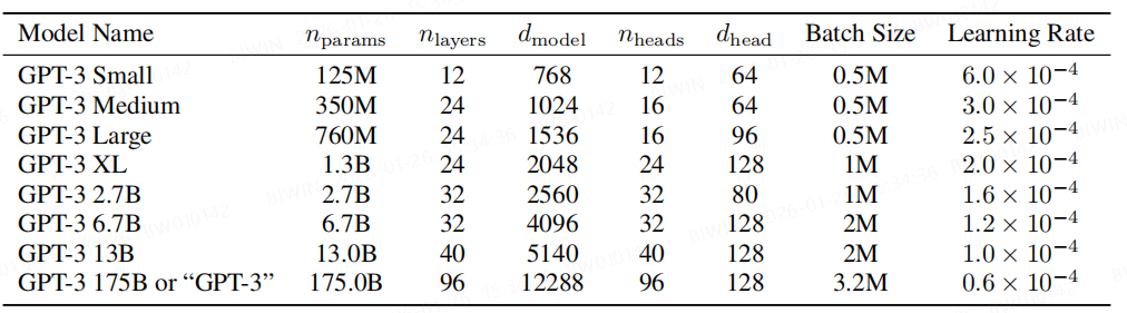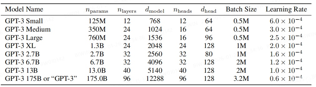


梯度更新

解释概念"gradient updates": 这里用线性回归的例子解释下，主要关注点是"**为了解决任务，模型参数需要更新才能更准确预测新情况**"。

用Python实现一个最简单的线性回归模型 $y=wx+b$(w: weight, b: bias)：

import numpy as np
import matplotlib.pyplot as plt
from matplotlib.animation import FuncAnimation

# 设置中文字体（可选）
plt.rcParams['font.sans-serif'] = ['SimHei', 'Arial Unicode MS', 'DejaVu Sans']
plt.rcParams['axes.unicode_minus'] = False

# 1. 创建一些简单的数据
np.random.seed(42)
X = np.array([1, 2, 3, 4, 5])  # 输入特征
y = np.array([2, 4, 6, 8, 10]) + np.random.normal(0, 0.5, 5)  # 目标值，加一点噪声

# 2. 初始化模型参数（权重和偏置）
w = 0.0  # 权重（初始值随便设）
b = 0.0  # 偏置
learning_rate = 0.01  # 学习率，控制更新步伐

# 存储训练过程中的参数变化
w_history = []
b_history = []
loss_history = []

# 3. 训练循环 - 这里就是梯度更新的地方！
epochs = 100  # 训练轮数

for epoch in range(epochs):
    # 前向传播：用当前参数做预测
    predictions = w * X + b

    # 计算损失（误差）
    loss = np.mean((predictions - y) ** 2)

    # 关键步骤：计算梯度（导数）
    # 这些梯度告诉我们参数应该往哪个方向调整
    dw = (2/len(X)) * np.sum((predictions - y) * X)  # 权重的梯度
    db = (2/len(X)) * np.sum(predictions - y)       # 偏置的梯度

    # 梯度更新：调整参数以减小损失
    w = w - learning_rate * dw  # 沿着梯度反方向更新权重
    b = b - learning_rate * db  # 沿着梯度反方向更新偏置

    # 记录历史参数
    w_history.append(w)
    b_history.append(b)
    loss_history.append(loss)

    if epoch % 20 == 0:
        print(f"Epoch {epoch}: w={w:.3f}, b={b:.3f}, loss={loss:.3f}")

print(f"\n最终模型: y = {w:.3f}*x + {b:.3f}")

# 4. 测试模型
test_X = 6
prediction = w * test_X + b
print(f"\n预测 x={test_X} 时，y ≈ {prediction:.3f}")

# 创建动画
fig, (ax1, ax2) = plt.subplots(1, 2, figsize=(15, 6))

# 左图：数据点和拟合直线的变化
ax1.scatter(X, y, label='真实数据', color='blue')
line, = ax1.plot([], [], 'r-', label='当前模型', linewidth=2)
current_point, = ax1.plot([], [], 'ro', markersize=8)
ax1.set_xlim(0, 6)
ax1.set_ylim(min(y)-1, max(y)+1)
ax1.set_xlabel('X')
ax1.set_ylabel('y')
ax1.set_title('线性回归训练过程 - 参数逐步优化')
ax1.legend()
ax1.grid(True, linestyle='--', alpha=0.6)

# 右图：损失函数随迭代次数的变化
loss_line, = ax2.plot([], [], 'g-', linewidth=2, label='损失值')
ax2.set_xlim(0, epochs)
ax2.set_ylim(0, max(loss_history)*1.1)
ax2.set_xlabel('迭代次数')
ax2.set_ylabel('损失值')
ax2.set_title('损失函数下降过程')
ax2.legend()
ax2.grid(True, linestyle='--', alpha=0.6)

# 动画更新函数
def animate(i):
    if i < len(w_history):
        # 更新左图：显示当前的拟合直线
        x_vals = np.linspace(0, 6, 100)
        y_vals = w_history[i] * x_vals + b_history[i]
        line.set_data(x_vals, y_vals)

        # 标记当前的最后一个数据点预测值
        current_y = w_history[i] * X[-1] + b_history[i]
        current_point.set_data([X[-1]], [current_y])

        # 更新标题显示当前参数
        ax1.set_title(f'线性回归训练过程 - Epoch: {i}, w: {w_history[i]:.3f}, b: {b_history[i]:.3f}')

        # 更新右图：显示损失函数变化
        x_loss = range(len(loss_history[:i+1]))
        y_loss = loss_history[:i+1]
        loss_line.set_data(x_loss, y_loss)

        return line, current_point, loss_line
    else:
        return line, current_point, loss_line

# 创建动画
anim = FuncAnimation(fig, animate, frames=len(w_history), interval=100, blit=True, repeat=True)

# 显示动画
plt.tight_layout()
plt.show()

# 如果需要保存为GIF文件，取消下面注释
# anim.save('linear_regression.gif', writer='pillow', fps=10)

在上面的代码中，**梯度更新**就是这两行：

w = w - learning_rate * dw  # 沿着梯度反方向更新权重
b = b - learning_rate * db  # 沿着梯度反方向更新偏置

什么是梯度？

• 梯度就是**导数**或**斜率**

• 它告诉我们：如果稍微改变参数（w或b），损失函数会如何变化

• `dw` 是负的 → 增加w会减小损失 → 我们应该增加w

• `dw` 是正的 → 增加w会增加损失 → 我们应该减小w

梯度更新的比喻：

想象你在山里蒙着眼睛找最低点（山谷）：

1. 你用脚感受地面的**坡度**（这就是梯度）

2. 你沿着坡度**向下走一步**（这就是梯度更新）

3. 重复这个过程，直到到达谷底（找到最优参数）

https://miro.medium.com/v2/resize:fit:640/format:webp/1*ohVPiStlsbMP0XL1_X-fkQ.gif

原文：

For all tasks, GPT-3 is applied without any gradient updates or fine-tuning, with tasks and few-shot demonstrations specified purely via text interaction with the model.

GPT-3没有梯度更新是什么意思？

1. **训练阶段**（已经完成）：

   • OpenAI用了45TB的文本数据

   • 训练了几个月

   • 进行了数百万次的梯度更新

   • 逐渐调整了1750亿个参数

   • 这个过程花费了数百万美元的电费

2. **使用阶段**（现在用的）：

   • 模型参数已经**冻结**了

   • 你输入文本 → GPT-3处理 → 输出回答

   • **整个过程没有改变任何权重参数**

   • 就像用计算器：你输入数字，它给出结果，但计算器本身不会改变

   • **这就解释了为什么说大模型没有记忆能力、知识滞后、无法自主更新**

代码类比：

class SimpleAI:
    def __init__(self):
        self.w = 2.0  # 假设已经训练好的权重
        self.b = 0.5  # 假设已经训练好的偏置
    
    # 训练阶段（已过去）
    def train(self, data):
        # 这里会有梯度更新代码
        # 但训练已经完成，我们不再调用这个方法
        pass
    
    # 使用阶段（现在）
    def predict(self, x):
        # 只是用训练好的参数做计算
        # 没有梯度更新！
        return self.w * x + self.b

# 使用训练好的模型
model = SimpleAI()  # w=2.0, b=0.5 已经固定

# 使用模型 - 没有梯度更新
print("预测 x=3:", model.predict(3))  # 输出: 6.5
print("预测 x=5:", model.predict(5))  # 输出: 10.5

# 注意：这里没有改变 model.w 或 model.b！
# model.w 还是 2.0，model.b 还是 0.5

由于大模型本身不具备”记忆能力“，而在实际应用中又往往需要其结合具体数据来生成回答，因此常会通过建立**数据库或知识库**来存储相关信息。当用户提出问题时，系统会先根据查询内容在数据库或知识库中检索与之相关的资料。随后，将检索到的信息与用户问题一并输入大模型，从而能够给出更准确、更具依据的回复。这类技术即属于大模型的衍生方向之一，例如检索增强生成（RAG）等。

few-shot


概念解释，原文:

(a) “few-shot learning”, or in-context learning where we allow as many demonstrations as will fit into the model’s context window (typically 10 to 100), (b) “one-shot learning”, where we allow only one demonstration, and (c) “zero-shot” learning, where no demonstrations are allowed and only an instruction in natural language is given to the model. 

优缺点，原文:

The main advantage of fine-tuning is strong performance on many benchmarks. The main disadvantages are the need for a new large dataset for every task, the potential for poor generalization out-of-distribution [MPL19], and the potential to exploit spurious features of the training data [GSL+18, NK19], potentially resulting in an unfair comparison with human performance.
...
The main advantages of few-shot are a major reduction in the need for task-specific data and reduced potential to learn an overly narrow distribution from a large but narrow fine-tuning dataset. The main disadvantage is that results from this method have so far been much worse than state-of-the-art fine-tuned models. Also, a small amount of task specific data is still required.

图说明：

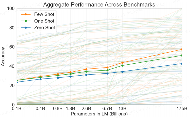
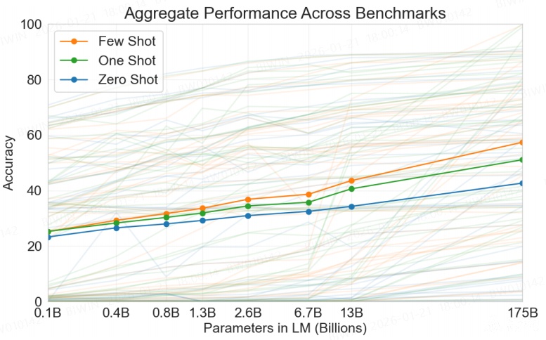
• 横坐标是模型参数

• 纵坐标是模型回答准确率

• 这张图是42个任务的评估表现，高亮的三条线是其中一个任务的结果，分别对应"Few Shot", "One Shot", "Zero Shot"

• 这张图说明了：

  • Few Shot 优于 One Shot 优于 Zero Shot

  • 模型参数越大，准确率越高


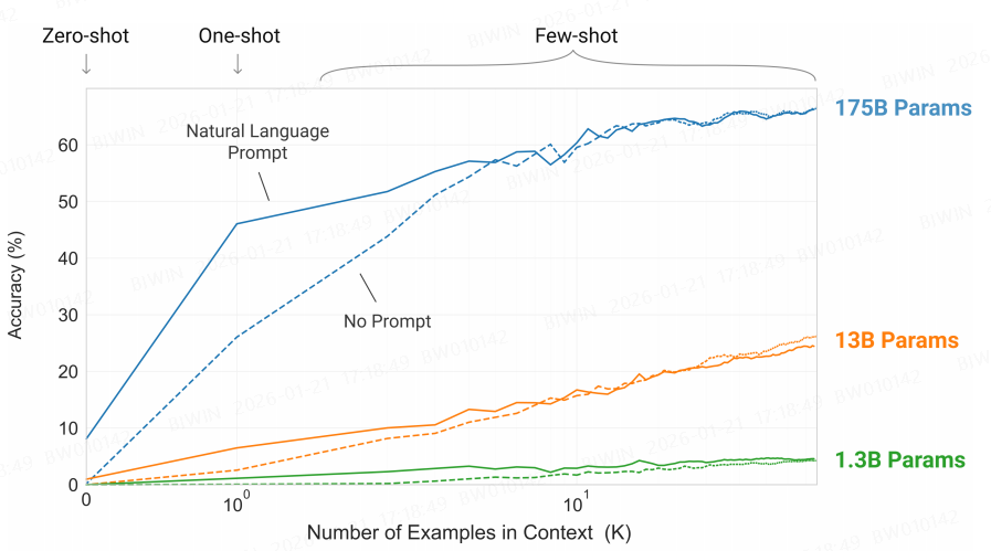
图说明（`a simple task requiring the model to remove random symbols from a word`）：

• 横坐标是例子数量

• 纵坐标是准确率

• 1.3B 模型，即使提供大量例子，准确率也很低；而175B则相反。说明few-shot learning能力需要模型参数足够多时才会出现（该现象称为「涌现」）

• 175B 模型，仅有抽象描述，准确率大概才10%，而提供一个例子后准确率接近50%。说明提供例子对准确率有直接的帮助

• 例子数量在$101$以下，有Prompt的准确率要显著高于没有Prompt。当例子数量超过$101$个以上后，即使没有 Prompt，准确率也与有Prompt一样高。


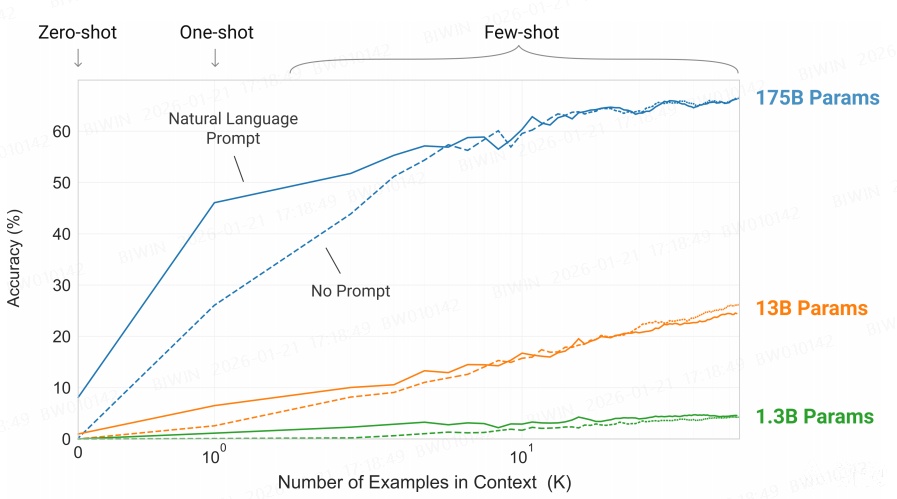
由此给出3点应用大模型的建议：

1. 通常情况下，参数量越大的模型能力越强

2. 要提供准确的抽象描述

3. 要提供具体例子，至少一个

原文:

Model performance improves with the addition of a natural language task description, and with the number of examples in the model’s context, K. Few-shot learning also improves dramatically with model size.Though the results in this case are particularly striking, the general trends with both model size and number of examples in-context hold for most tasks we study. We emphasize that these “learning” curves involve no gradient updates or fine-tuning, just increasing numbers of demonstrations given as conditioning.

优点


大量的训练数据 -> 已具备诸多技能。例如，大模型本身就具备了翻译能力。

原文：

whereas translation clearly must be learned during pretraining, although possibly from data that is very different in organization and style than the test data

无需额外的训练，无需大量的数据，**仅仅需要调整文本**，提供少量的几个例子，就可以解决全新的NLP任务。

而传统的机器学习，要解决某个NLP任务，都要大量的数据和训练模型，适用范围窄。

原文：

from a practical perspective, the need for a large dataset of labeled examples for every new task limits the applicability of language models. There exists a very wide range of possible useful language tasks, encompassing anything from correcting grammar, to generating examples of an abstract concept, to critiquing a short story. For many of these tasks it is difficult to collect a large supervised training dataset, especially when the process must be repeated for every new task.

特点：训练成本高，部署/使用成本低 (随着技术发展，大模型的能力会更强，还更便宜)
注意：训练成本高不只指显卡、电费这些硬件成本，数据的筛选、标注、处理等也是极高的成本。

原文：

Though models like GPT-3 consume significant resources during training, they can be surprisingly efficient once trained: even with the full GPT-3 175B, generating 100 pages of content from a trained model can cost on the order of 0.4 kW-hr, or only a few cents in energy costs.

缺点

训练的数据多，既带来了知识量大的优点，也可能导致学会了一些偏见.

6.2 Fairness, Bias, and Representation

仅具备语言知识，不具备世界知识、物理知识。因此，会出现“幻觉”现象。

large pretrained language models are not grounded in other domains of experience, such as video or real-world physical interaction, and thus lack a large amount of context about the world

大模型可能会产出假消息，不可全信。

we find that GPT-3 can generate samples of news articles which human evaluators have difficulty distinguishing from articles written by humans.

训练

• https://www.bilibili.com/video/BV1MY4y1R7EN

GPT的本质是：predict next token，也就是”单字接龙“。

https://github.com/jingyaogong/minimind/blob/master/images/1-wiki.png


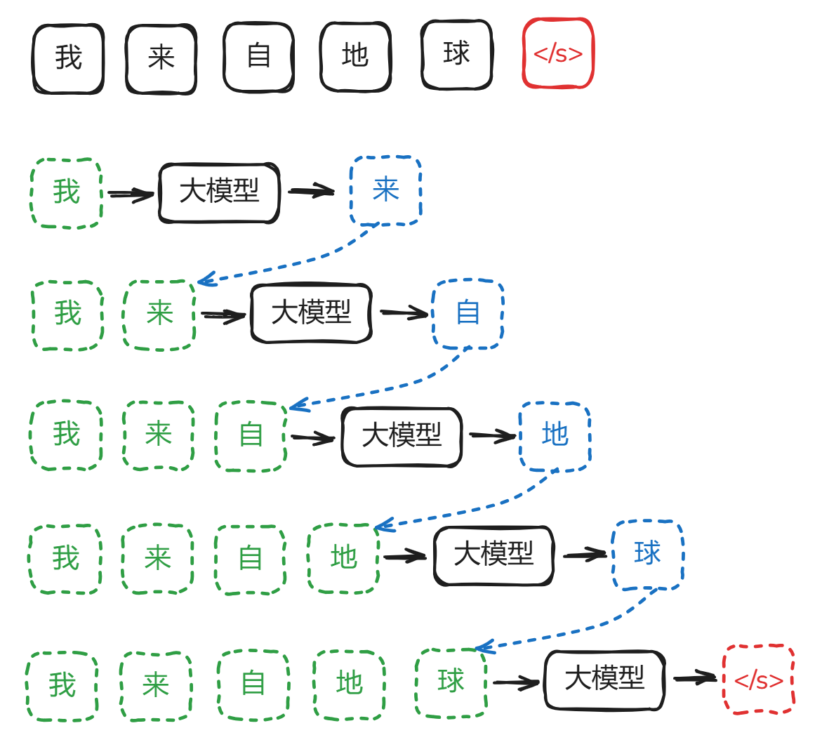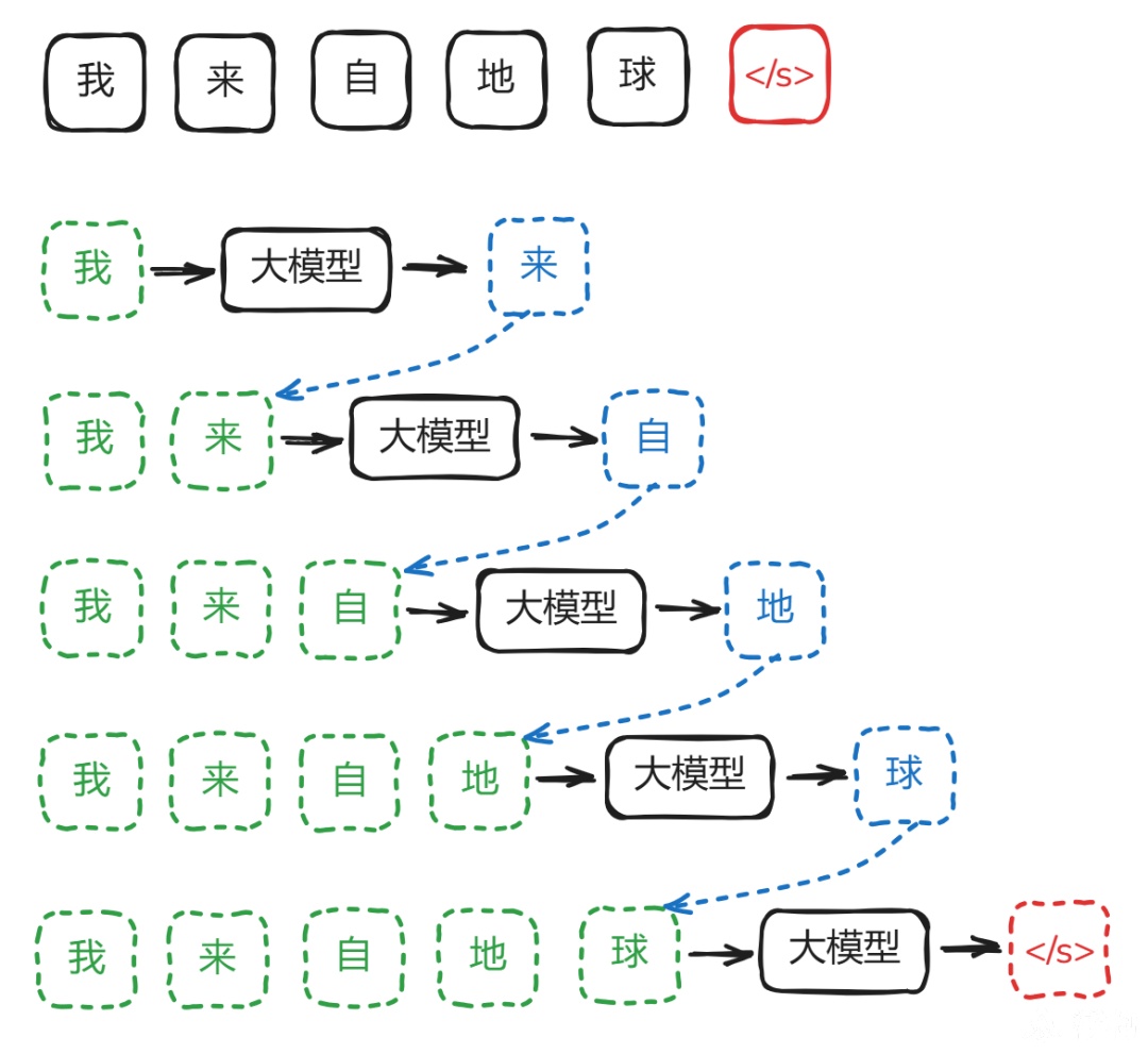
训练资料：”我来自地球“。
训练时：

• 大模型输入：”我“，要求输出：”来“

• 大模型输入：”我来“，要求输出：”自“

• 大模型输入：”我来自“，要求输出：”地“

• 大模型输入：”我来自地“，要求输出：”球“

• 大模型输入：”我来自地球“，要求输出：结束符号

应用时：
大模型其实只能输出一个字，只要把输出的字与上文结合形成新的上文，就可以再生成新的一个字。不断循环这个过程，也就能生成任意长的下文了。这个过程叫”自回归生成“(autoregressive)。这也解释了为什么大模型输出时，是逐个字逐个字输出的。

训练资料很多，可能不止”我来自地球“，还可能会有”我来自中国“等语句。因此，大模型的输出其实不是固定的，而是字的概率分布。假如说，输入是”我来自“，输出是”地“的概率是10%，输出是”中“的概率是60%，其它字总共的概率是30%。简单来说，问10次”我来自“，大模型有1次回复”地“，有6次回复”中“，另外3次回复的是其它字。这就解释了为什么，同样的文本输入，大模型可以产生不同的回答。

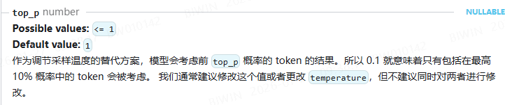
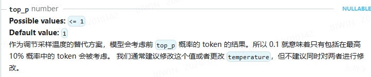
扩展：在调用大模型api时，会提供一个 top_p 参数，可以用来调控模型输出的随机性。

https://api-docs.deepseek.com/api/create-chat-completion


为什么采用逐个生成(Autoregressive)，而不采用一次性生成全部(Non-autoregressive)的做法呢？

还是上面的例子，输入是”我来自“，可以回答”地球“或者”中国“。
如果采用 Autoregressive，假设先生成”地“，则下一字是”球“的概率就会比”国“的概率高很多。
如果采用 Non-autoregressive，第一个生成了”地“，第二个可能生成为”国“，也就导致生成”我来自地国“这种奇怪的说法。

这只是GPT的训练原理，还有一些训练步骤才形成当前使用的大模型，如，有监督微调(Supervised Fine-Tuning)，知识蒸馏 (Knowledge Distillation, KD)，训练推理模型 (Reasoning Model)，等等。

原文：

For all these reasons, scaling pure self-supervised prediction is likely to hit limits, and augmentation with a different approach is likely to be necessary. Promising future directions in this vein might include learning the objective function from humans [ZSW+19a], fine-tuning with reinforcement learning, or adding additional modalities such as images to provide grounding and a better model of the world [CLY+19].

其它

在理解其学习原理后不难发现，现在的大模型还不至于网上传闻的那么“神奇”。从本质上说，它只是一个工具，只是一个运行在计算机里的程序，没有意识没有欲望没有情绪，并不具备主动取代人类的能力。

这就像自动驾驶服务“萝卜快跑”，虽然具备自动驾驶功能，但它的行驶完全取决于人的指令——只有当人需要时，它才会从A地行驶到B地。同样地，大模型本身并不会主动创造内容，它的“智能”本质上是对海量数据中统计规律的复现与组合。只有当我们提出明确需求时，它才会基于这些规律生成相应的文字，其产出完全由人的意图所驱动。

这种工具属性是由其根本原理决定的。大模型并不真正“理解”文字的含义，而是通过概率预测下一个最可能的词。因此，其输出始终围绕给定的上下文展开，既没有自主意识，一切作用最终都取决于人如何使用它。

日常交流中，不要仅仅讲抽象描述，最好多讲一些具体例子，哪怕只有一个。

原文:

In some cases it may even be difficult for humans to understand the format of the task without prior examples, so this setting is in some cases “unfairly hard”. For example, if someone is asked to “make a table of world records for the 200m dash”, this request can be ambiguous, as it may not be clear exactly what format the table should have or what should be included (and even with careful clarification, understanding precisely what is desired can be difficult).